Viola-Jones Algorithm – Detecting Faces in Just a Few Lines of Code

Face detection is an established computer vision task concerned with finding one or more faces in a given image. If you open your phone’s camera, there is a high chance that some sort of face detection technique is being used to detect faces. With significant advancements in deep learning technologies, computers can now detect and recognize faces quite accurately. But there is always some trade-off between speed, accuracy, complexity, and efficiency.

But before all the flashy face detection techniques were in mainstream, In the year 2001, two computer vision researchers Paul Viola and Michael Jones, proposed a framework in their paper, “Rapid Object Detection using a Boosted Cascade of Simple Features”, which was a breakthrough in this field although having ability to be trained to detect a variety of objects but mainly motivated by the problem of face detection.

Despite being an old framework, the Viola-Jones algorithm is a rather powerful, fast, and robust algorithm for detecting faces (not recognizing). The drawback of this algorithm is that it requires fully frontal upright faces to be detected successfully. A tilted face, half face in the frame, etc., can hurt the algorithm's utility. But given that detection is usually followed by a recognition step, the limitations on poses are acceptable. Also, it is pretty slow to train. But as we will see further, the algorithm makes up for its drawbacks with the speed at which it detects the face.

Algorithm Under the Hood

The algorithm works in four stages:

1. Selecting Haar-like Features
2. Creating an Integral Image
3. Running AdaBoost Training
4. Creating Classifier Cascades

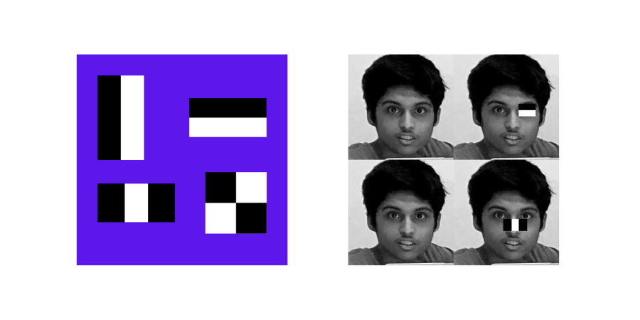
Haar-like features get their name from having a striking similarity with Haar Wavelets’ concept, given by a Hungarian Mathematician in the 19th century and used in the first real-time face detector. Human faces share a universal property of having dark and light neighboring components like eyes that begin darker than the upper cheek. These universal properties are the Haar-like features that Viola-Jones Algorithm exploits to get the task done.

Using these features, the algorithm interpreted parts like nose, cheeks, etc. The value of the feature is calculated as a single number: the sum of pixel values in the black area minus the sum of pixel values in the white area. The value is zero for a plain surface in which all the pixels have the same value and thus, provide no useful information.

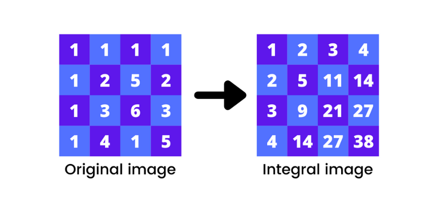
An integral image adds up all the pixels above and to the left of the target pixel with its value. Calculating values for each feature can be computationally expensive if we are dealing with a large feature. The integral image helps compute these values in constant time, giving a considerable boost in the speed.

AdaBoost is a popular Machine Learning algorithm that helps in efficiently choosing the best features among a large number of possible features (160,000+ features can be in just a 24 x 24 image). After this step, we get a strong classifier called the boosted classifier with a significantly reduced work time.

Cascading Classifier discards the pixels without human faces. On average, only 0.01% of sub-windows are positive, meaning they probably have a facial feature in them. It is better to filter out the negative windows in the first layer and spend more time on the positive ones. Therefore, in a cascaded architecture, the 1st layer acts as a filter removing negative windows and transferring the windows with above 50% possibility of having a facial feature to the next layer. The next layer looks for the negative windows more strictly on the windows that survived in the first layer, and the process goes on until we reach the final stage.

Detecting Faces in Just a Few Lines of Code

Now that we know the Algorithm let us try to detect faces in a given image using the Viola-Jones Algorithm.

We will use the OpenCV python library, so if you don’t have it already, you can download it by simply running the following command from your command prompt or Terminal pip install opencv-python.

Let's import libraries to be used:

1. import os
2. import cv2

From here, we will need to load the viola jones classifier called the Haar Cascade Classifier. There are two ways to do it. The Haar cascade classifier for the face and numerous other classifiers comes along with the OpenCV package you just downloaded. You can view that by navigating to the folder where your OpenCV is located and then going into the data folder. In case you don’t know where your OpenCV package is located, here is an easy trick:

import cv2 print(cv2.file)

Run the code, and you will get a path as output. Change directory to the output path, and you will see something like this:

In the data folder you will find all the different Haar-cascade classifiers for face, eyes etc in XML format. Even after this if you are facing any errors, we are including the classifier XML file that you can download and use directly.

Now let’s get the path of our classifier and load our classifier:

CODE

cv2_base_dir = os.path.dirname(os.path.abspath(cv2.__file__))
haar_model_face =
os.path.join(cv2_base_dir,'data/haarcascade_frontalface_default.xml')
face_detector = cv2.CascadeClassifier(haar_model_face)

Load the Image:

CODE

img = cv2.imread(“image.jpg”)

Detect Faces:

Convert image to grayscale

CODE

gray = cv2.cvtColor(frame,cv2.COLOR_BGR2GRAY)

Detect faces

CODE

face_detector.detectMultiScale(gray,scaleFactor=1.1,minNeighbors=2,minSize=
(50, 50),flags=cv2.CASCADE_SCALE_IMAGE)

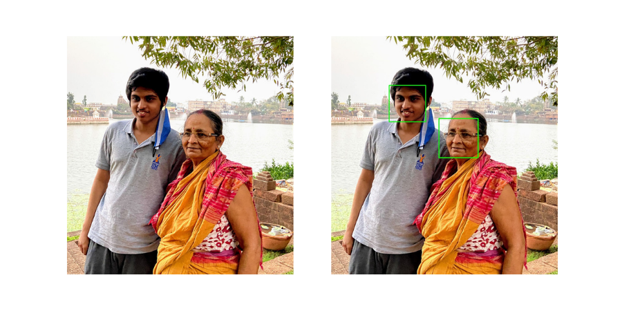
That’s it; that’s all we needed to detect faces. The last step will be to draw the rectangles around the faces in the image.

Here is the final code:

CODE

import os
import cv2
# Getting the path of the Haar-cascade classifier
cv2_base_dir = os.path.dirname(os.path.abspath(cv2.__file__))
haar_model_face =
os.path.join(cv2_base_dir,'data/haarcascade_frontalface_default.xml')

Loading the detector

CODE

face_detector = cv2.CascadeClassifier(haar_model_face)
# Loading the image
img = cv2.imread(“image.jpg”)

Convert image to grayscale

CODE

gray = cv2.cvtColor(img,cv2.COLOR_BGR2GRAY)
# Detect faces
faces=face_detector.detectMultiScale(gray,scaleFactor=1.1,minNeighbors=2,minSiz
e= (50, 50),flags=cv2.CASCADE_SCALE_IMAGE)

Drawing bounding boxes

CODE

for (x,y,w,h) in faces:
cv2.rectangle(img,(x,y),(x+w,y+h),(0,255,0),2)

Displaying

CODE

cv2.imshow(“Window”,img)
cv2.waitKey(0)

Output