Computer Vision with Python OpenCV

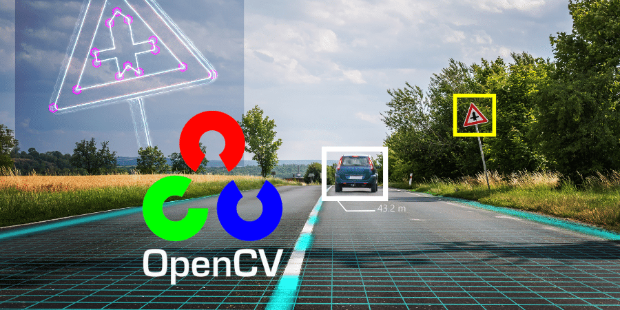
OpenCV is an Open Source library with tons of in-built functions that makes image and video processing tasks and real-time computer vision much more effortless. It supports various programming languages like Java, Python and C++ among others, and operating systems like Windows, Linux and macOS. All functions of OpenCV are written in C/C++ to take advantage of multi-core processing. OpenCV, combined with libraries like NumPy, becomes even more powerful by allowing us to treat images as a matrix and even apply mathematical operations.

Installing OpenCV for Python

Open up your cmd or terminal and write the following commands:

pip install numpy
pip install opencv-python

How Does a Computer See an Image?

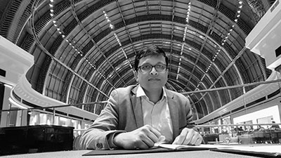
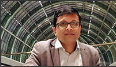
When you look at the below picture, you can quickly identify what it is. It often doesn’t make sense why a computer cannot do that? This is simply because computers can’t see the image as we do. It can’t make sense of the images. Let's see how a computer sees an image to make it clearer.

We can load an image using OpenCV imread() function. The syntax of cv2.imread() function is given below:

cv2.imread(path-to-image, flag)

where the path to an image has to be the complete path or relative path to the image on the machine. The flag is optional.

import cv2 #importing opencv
import numpy as np #importing numpy
img = cv2.imread('ashwini-image-grayscale.jpg', 0)
print(img)

As you can see, the output is just a 2D array of numbers. Which to be honest doesn’t even make much sense to us. Every cell in the matrix is a pixel so since the image was 400x225 the matrix is also 400x225. Each cell accepts an 8-bit value that means from 0-255. You can also check the size by using the shape method.

img.shape

(400,225)

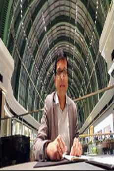
Colour Images

In the above example, we used a grayscale image now let's see what is different with a coloured image.

import cv2 #importing opencv
import numpy as np #importing numpy
img = cv2.imread('ashwini-image-color.jpg')
print(img.shape)

(400,225,3)

As you can see, there is an extra 3 in the shape and it's a 3D matrix instead of 2D. The first value is the height of the image, second is the width of the image. The third value is actually the channels of the image. Each cell of the matrix or the pixel of the image now has three primary colours Blue(B) Green(G) Red(R) - each of 8-bit value 0-255. One thing to note is that OpenCV reads an image as BGR by default and other libraries like matplotlib read it as RGB by default.

Displaying an Image

We can also display the image in a window. It is done by cv2.imshow() function

cv2.imshow(window-name,img)

The 'window name' is just the title of the window in which the image is displayed. 

img is the image that we loaded using OpenCV

import cv2
img = cv2.imread('ashwini-image-color.jpg ')
cv2.imshow('example window',img)
cv2.waitKey(0) # waits until a key is pressed
cv2.destroyAllWindows() # destroys the window showing image

Different Colour Channels of an Image

There are many types of colour channels like grayscale, BGR, RGB, HSV, CMYK, Alpha etc. - RGB/BGR and grayscale in the above examples. Each channel has its own advantages and usage.

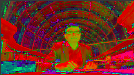
Converting from One Colour Channel to another

Let us convert from RGB to HSV (hue, saturation, value)

img = cv2.imread('ashwini-image-color.jpg ')
img_HSV = cv2.cvtColor(img, cv2.COLOR_BGR2HSV)
cv2.imshow('hsv-image-example', img_HSV) #show image
cv2.waitKey(0) # waits until a key is pressed
cv2.destroyAllWindows() # destroys the window showing image

Manipulating image

import cv2
import numpy as np
img = cv2.imread('ashwini-image-color.jpg ')

A. Scaling an image

image_resize=cv2.resize(img,(200,300))
cv2.imshow(resized image',image_resize)
cv2.waitKey(0)
cv2.destroyAllWindows()

B. Cropping image

Since the image is a matrix, the cropped image is just a sub-matrix of the image  

height,width = img.shape[:2]
start_row_idx,start_col_idx = 100,50
end_row_idx,end_col_idx = 300,170
image_cropped = img[start_row_idx:end_row_idx,start_col_idx:end_col_idx]
cv2.imshow("new image after cropping”, image_cropped)
cv2.waitKey(0)
cv2.destroyAllWindows()

Mathematical operations

Adding and subtracting value to and from all the pixels

matrix = np.ones(img.shape, dtype="uint8") * 50
img_add=cv2.add(img, matrix)
cv2.imshow("image with added values", img_add)
cv2.waitKey(0)
img_subtract =cv2.subtract(img, matrix)
cv2.imshow(" image with subtracted values ", img_subtract)
cv2.waitKey(0)
cv2.destroyAllWindows()

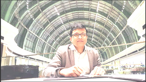
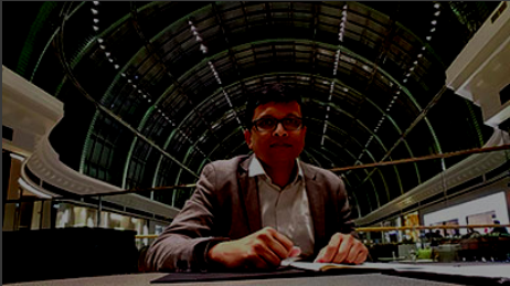
Observe how the brightness changes when we add or subtract value from a pixel.

 Writing an Image to Disk

cv2.imwrite(img-path,img)

Let’s quickly see a code to read an image, scale it and finally write a new scaled image to disk

import cv2
import numpy as np
image=cv2.imread('ashwini-image-color.jpg ')
img_resized = cv2.resize(image,(500,500))
cv2.imwrite("ashwini-image-color-min.jpg",img_resized)

Conclusion

As we said at the start of the article, a computer cannot make sense of images. It's a problem the computer vision algorithms are trying to solve. The idea is to teach a computer how to make sense of a matrix of numbers and identify objects, faces and characters using mathematical principles. The newer techniques are becoming better and better every day. This is being integrated into our daily lives in the form of technologies like self-driving cars, Google reverse image search, etc.