 Batoi Corporate Office
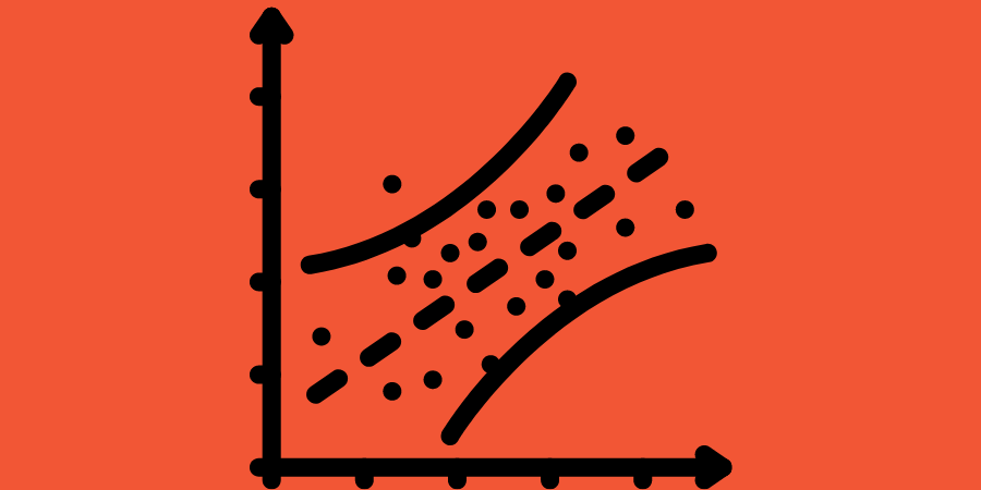
Linear regression is a statistical model for making predictions using several variables to explain what happens in a process or system. When you create a linear regression model, you fit a line (or curve) to the data. The line that best fits the data is selected, and you can use this line to make predictions. Because the number of variables is usually more than one, and these variables indicate something about a system, linear regression models are essential tools in physical science (sometimes called multivariable models). Linear regression has been used since 1880, when it was developed by Francis Galton, though it has also been independently developed in several other places.
If you are new, the above definition might not have made much sense. So let’s try to understand it with a problem statement. The problem statement is called “Predicting housing prices”. It is a famous regression problem used to get started with linear regression and other more complex regression models.
We have a dataset with key-value pairs. The key represents the square footage of the house, and the value represents the price of the house.
The task is to train a model such that when given a key (square footage of the house) that was not present in the dataset earlier, the model can predict an approximate price of the house. See the following graph:
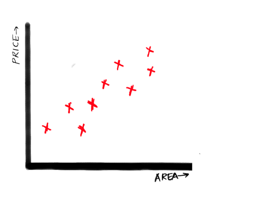
The x-axis represents the square footage of the house, and the y-axis represents the price of the house.
If you observe carefully, the price is increasing kind of linearly with the increase of the square footage. So if we can draw a straight that passes just like shown in the next graph:
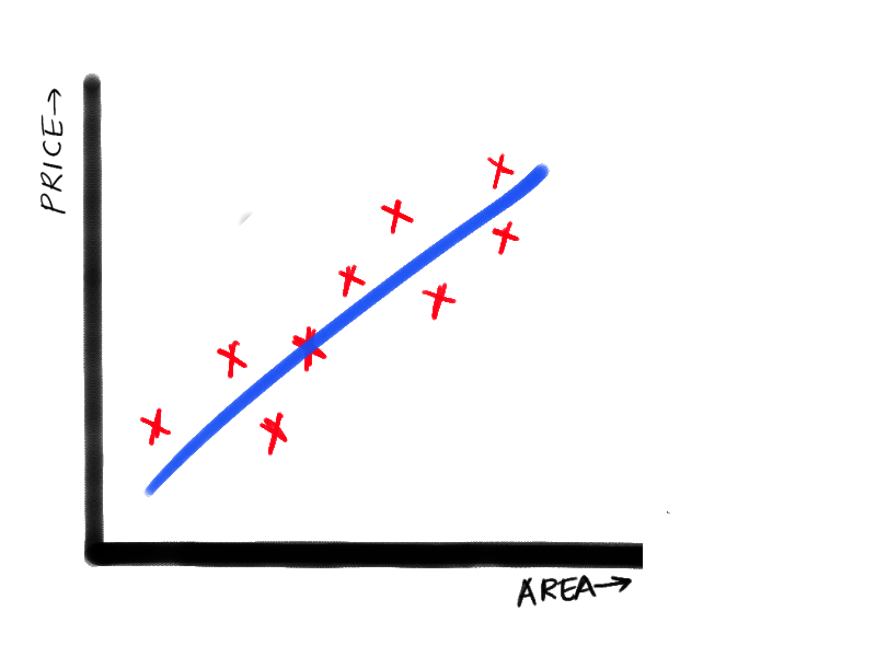
This line doesn’t pass through all the points exactly, but this line can be extended infinitely, and the prices of the house, given any square footage, can be calculated. Now the question arises, “Why this line? Why not some other line, maybe with more slope or less slope? What unique property does this line have?” The answer is “minimum error”. You see, the difference in the approximated value that this line is predicting an exact value that we have from the data set can be used to calculate the error. And if we can minimize the overall error, we can make a reasonable prediction. And this is how the supervised learning model works. We have a hypothesis (like the linear relation in this problem statement). We try to train a model based on this hypothesis such that the error we get is minimum which in turn means the accuracy is maximum.
The Hypothesis
As we saw, the hypothesis here was that the output varies linearly with the input. Mathematically it looks like this:
You might also know it as the equation of the straight line. Here a, b are the parameters that are unknown to us. If we somehow find out their values, we can draw our line. This is where the learning of the supervised “learning” or rather machine “learning” comes in. During the training phase of the model, it tries to figure out the values of these parameters by itself. So if you ever wondered how or what the machine learning model learns, this is it.
Training Our Model
So how do we start training our model? Let’s start with some random values of a and b. Say 5 and 8. If we put that in our function, it becomes:
As we can see, the first data point in our dataset is (x0=2104,y0=460). If we put them in our function, we get y(x0)=16837. We can already see that we didn’t get y0 which was our desired output. There is an error. And we are going to use this error to train our model.
The Error Function
We know there is an error, but how do we use it. The error is calculated using an error function or the cost function. There are many different error function out there that you can read about. Here we are going to use something called mean squared error. This is relatively simple as it just squares the difference between the actual and predicted value to calculate the error. And to calculate the final error, we just average out the errors for all our data points. Mathematically it looks like this:
Where ‘m’ is the total number of data points.
Now the last step is the optimization step.
Optimization
The optimizer function is a function that we use to update the values of the parameters. The optimizer that we are using here is called gradient descent. The updating of the parameters looks like this:
We are not going to get into how this optimizer works in this article. We will learn about it in more detail in some other article.
"Alpha" here is called the learning rate. This is another parameter that we need to adjust ourselves. Some common values for learning rates include 0.1, 0.01, 0.001, and 0.0001.
After we have updated the parameters, we again follow the same steps, and we keep on doing this until we minimize the overall error.
Uses of Linear Regression
Linear regression is used extensively in the social sciences, where it has been shown to have a valuable number of applications, such as predicting outcomes and testing hypotheses. Linear regression is a handy tool for data analysis. It allows us to quickly explore relationships in the data, gain insights into various aspects of that relationship, and make predictions based on those insights. All of this can be achieved with just a basic knowledge of matrix algebra and assumptions about the relationships in the data - no regressions or partial differentials required.